Onfleet leverages machine learning to produce best-in-class real-time predictions for driver arrival and delivery completion time. At peak, we maintain estimates for tens of thousands of deliveries in real-time.
Overview
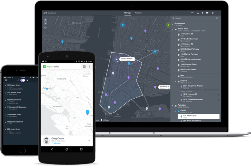
Onfleet is a platform for efficient management of local delivery. We manage deliveries for hundreds of businesses in over sixty countries around the world. Our customers use an in-house fleet, outsource through a partner, or use a hybrid model within or between cities.
The basic primitive in Onfleet is the task, which is a request for a driver to go to a single location. By leveraging dependencies, more complicated operational models are accommodated (e.g. pickup-dropoff, hub-and-spoke, long routes). Having powered tens of millions of tasks for hundreds of businesses around the world, we are able to leverage an immense amount of aggregate data to improve the platform and drive operational efficiencies for all of our customers.
This article is focused primarily on the prediction of task completion times and does not cover other features of the Onfleet platform, like notifications, our real-time dashboard and driver app, or other tools for optimization and analytics. Check out our Features page to learn more about other features of the platform.
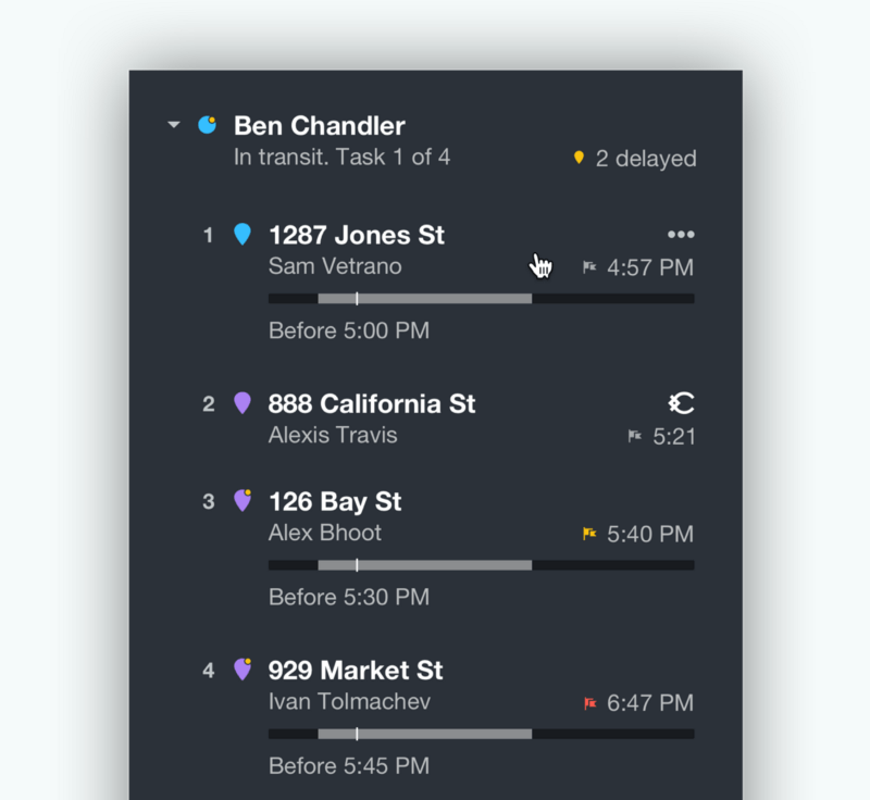
We perform multiple types of predictions in real-time. We compute ETAs for active tasks which are shared with the task’s recipient as well as estimated completion times (ECTs) for all assigned tasks. ECTs are available to a dispatcher through the dashboard and API and are used to derive additional operational information. An ETA is an estimate of when a recipient should be ready for the driver to arrive while an ECT is an estimate of when a driver will be done picking up or dropping off an item, ready to perform the next task. Without other constraints, we assume tasks will be completed as soon as possible by a driver; to indicate that a task should be completed after a certain time, a completeAfter time may be specified. Its counterpart, the completeBefore time, is often used when a promise is made to a customer to complete a delivery by a certain time. We use this property to surface information about how delayed a task is and to provide analytics to businesses. We also consider service time, the time spent by the driver reaching and interacting with the customer. A serviceTime value may be specified explicitly for a task which will override our prediction. This is useful, for example, for a restaurant delivery service for which external factors like food preparation time must be accounted. Now, let's dig in.
Simplifying assumptions
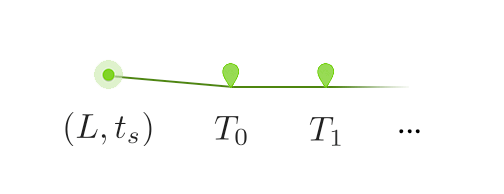
Let’s make a few simplifying assumptions to narrow the scope of this article. Notably, let’s keep it simple by exploring how a system can work without needing to consider schedules or dependencies. We’ll explore how estimation works for a driver who is online now and ready to perform deliveries, treating all deliveries equally and only estimating the ECT for all tasks T_i. We’ll call such a list of tasks a route. In this model, we will assume that the driver starts at a location L at time t_s and then will complete the tasks T_0, T_1, … in order.
A simple downstream model
To begin, let’s relate the completion times for task i, C(T_i), to an estimate of the duration of each task and to the completeAfter values corresponding to each. We refer to this relationship between duration and completion times as a downstream model. Note that all estimates will vary in time since our estimates change over time; this condition will soon be addressed.
We’ll start with the completion time for task T_0. We’ll assume the current time is t_s. On first pass, since the driver is starting immediately, we can simply add the duration of the task, dur(T_0; t_s) to determine the completion time C(T_0) = t_s + dur(T_0; t_s), however we still need to account for the completeAfter; in this case, the driver can’t leave any earlier so this constraint can only delay the task as

where C_a represents the completeAfter time for a task. For convenience, we’ll let C_a =-∞ if unspecified. One lingering detail here is why we can run our duration model starting at t_s, even if the task actually starts later due to a completeAfter time. Let’s consider the cases. If the task is completed before the completeAfter, the task must be achievable before this time and so we can use the completeAfter safely. On the other hand, if it’s completed after, we’ll start immediately and the completeAfter has no effect. As such, we only need to model duration on the start time of a task to determine the completion time, even if the task will actually start between these two times.
Now that we have a simple model for one task, we can easily extend this model to multiple tasks. Since we know when a task will complete, we can feed this time into the same equation for the next task, arriving at our general formula,

where we notionally let C(T_-1) = t_s for convenience.
In a toy system, we would simply need to determine the duration for each task to run this operation over a set of deliveries. This approach is infeasible at scale, however, since it requires many estimates of duration. If the average on-duty driver has even five tasks and changes location once per second, with memoization we would still need to perform five evaluations per second per driver. For a cheap model, like a simple relationship between straight-line distance and duration, this is perfectly acceptable but it would become computationally expensive for a more sophisticated estimator. With thousands of drivers and routes which may exceed 50 tasks, we need a better approach.
In practice and at scale
In practice, we receive hundreds of locations per second. Additionally, we need to update tasks whenever the driver’s task list changes, as new deliveries are added or adjusted, or as the real world changes. While a naïve approach would be infeasible, we can reduce this computational burden. We maintain estimates for all tasks by using an invalidation mechanism to propagate the invalidations forward when a difference exceeds a threshold from the previous computed value. As such, we are often able to update a fraction of the tasks on any update which might affect them, practically around 2%. This reduction is equally owed to the relative stability for the duration of the average task over short time ranges and to the effect of completeAfter times. We allow for back-pressure naturally by using a set-like invalidation queue, where a route can only have one in-flight invalidation. This is important when bulk operations affect many drivers in a short time-frame. This means we often only need to evaluate our duration model tens of times per second instead of thousands.
What about estimation?
All of the above glosses over the meat of the problem: how we can estimate task duration in the first place. Let’s set the stage. We know the previous location where a driver starts and where the task will end. We also can assume a start time for the task. Then, the goal of a model is to predict the duration. Practically, we also know other details about the task: which organization has created it and other metadata signifying its operational role, for example.
Learning an end-to-end model for such a problem is tricky and we tackle it by separating it into sub-problems. Since we collect data at a high temporal frequency, we can implement other algorithms to post-process task locations to determine different phases of the task: the period before driving begins, the driving portion of the task, and the parking and service time. Then, we split duration into several different parts,

where we let T_b be the average time a driver spends finishing one task and preparing for another, TT(•) be the transit time, and ST(•) capture the service time. Note that the service time may be overridden when running the estimator, as previously mentioned.
T_b is relatively easy to learn as we can start with a simple mean and trend toward better estimates as more data become available for the organization and driver.
Learning an end-to-end machine learning model for transit time is something we call “pseudo-routing”, where we estimate the duration for a task given the start and end location, start time, and other operational parameters. In practice, we actually estimate a distribution over the transit time as well as the traveled distance. The most salient features for this task are the time-of-day, the day of the week, and the start and end locations. In practice, other features are added to improve the accuracy. Of these, location is the most challenging. A toy model can be constructed simply by gridding the world but this results in accuracy close to neighborhood level in areas with many examples and may produce nearly empty cells in others. We use several novel techniques to address this problem, allowing for precise location information to be captured naturally in places where sufficient data exists. While I’d love to elaborate, the margins of this article are simply too small to contain an explanation.
Finally, let’s consider the problem of service time estimation. This can be achieved in a similar way to transit time estimation and also takes into account features for the organization and task metadata. Location can be surprisingly important for service time; for example, it may take significantly longer to park in a dense urban area than in a suburb. This effect is also time-based. Of most relevance with regard to metadata is whether the task is a pickup or dropoff task. To illustrate, picking up items from a warehouse often takes significantly longer than dropping them off at a residential address. This variable has a strong interaction with the organization since different organizations have different operational models.
Learning is often constrained by access to data. We have powered over ten million deliveries, which gives us enough data to produce reasonable results. Further, for some tasks like transit time estimation, there exist reasonable forms of data augmentation since transit can be divided into smaller chunks to yield many more examples.
As a final note on the topic of estimation, these kinds of models are best for applications where the models are stateless. An online model is often better suited for a task like the estimation of an ETA once a driver is en route. For example, an online model can adjust estimates based on observed driver speed independent of other reported traffic flow rates or historical data, which often produces a moderate improvement in accuracy. As such, Onfleet uses a separate online model for estimation of ETAs.
Future work
There are many avenues to improve our models. We assume all drivers in an organization spend equal amounts of time during the service time phase, for example. There are additional features which may be added to improve accuracy. Perhaps weather information is the most germane. While this is being considered, it is constrained by access to high-quality global historical weather data for the time being.
Aside from improving and tuning our models, there are a few higher-level improvements in the pipeline at Onfleet. Notably, we plan to introduce features to better couple tasks with an operational relationship and to build a hybrid system for estimation of transit time, blending ML with open data.
For the former, as previously alluded, this form of downstream model doesn’t naturally account for dependencies or other task relationships. We currently use a simple approach to build them in but more sophisticated models may be considered. For example, a driver is not necessarily occupied during the preparation of food and so the service time for a pickup task may occur during transit; there’s no need to assume the driver needs to wait for it to complete. These types of modifications may be captured by altering the downstream model to build in this variation; for example, we can propagate a time range through our downstream model instead of a single time.
Using an end-to-end ML system for transit time is attractive in its simplicity but doesn’t exploit all accessible knowledge about the world. A next-generation system would combine open data like OSM lane restrictions with ML using a hybrid routing system. We use a pure ML model as it has advantages like intrinsically learning variation in road speed by time of day and day of week or learning how road structures or traffic flows change over time. With significantly more data (on the order of billions of deliveries and trillions of locations), this approach may begin to overtake classical routing using estimated road speeds but for now a hybrid approach is most promising for us. In this way, we can take advantages of an ML model within the framework of routing over open data.
Finally, while prediction comes with intrinsic utility, it’s often most useful when it can be acted upon. In complement to our prediction of task completion times and delays, we’re working on tools to optimize deliveries in real-time over these estimates to continue to deliver the best results as the world changes. Stay tuned!
Conclusion
Modeling the future in the world of local delivery is challenging. We’ve only just begun on the journey of accurate prediction. The space contains many hard problems and open data often misses low-level details which are revealed through a high-quality, in-domain dataset. Our goal is to produce the most efficient, transparent, and delightful delivery experience for our customers.
If you like machine learning, delivery, geo-data, or other topics mentioned here, stay tuned and feel free to reach out. If you’re managing delivery operations using your in-house software or another platform, we’d love to chat about how we can work together to deliver the most value for your business.